Amazon Redshift ML - Creating Machine Learning Models with Standard SQL.
Using SQL to predict telecoms customer churn based on customer activity data (95+% accuracy).
The term Machine Learning is no longer just a marketing buzzword for tech products. Nowadays, it is the brain behind the scenes making intelligent predictions on the majority of application and software solutions that we interact with on a daily.
At AWS re-Invent 2020, the AWS team announced the preview release of a machine learning feature for Amazon Redshift known as Amazon Redshift ML. Now that the feature is generally available for all AWS regions, I decided to take it for a spin by testing how accurate this feature is at solving common ML problems (starting with a simple BinaryClassification problem).
This article goes through a step-by-step procedure of using standard SQL to create and train machine learning models within an Amazon Redshift database.
Building ML Model with Redshift ML
Redshift ML is an Amazon Redshift feature that makes it easy for data scientists, engineers, or developers to create, train, and apply machine learning models using just SQL (no other tool or language is needed).
Training of a machine learning model using Redshift ML is powered by Amazon SageMaker, a fully managed machine learning service that is also available on the AWS platform. Sagemaker is able to detect patterns from provided dataset to create a model.
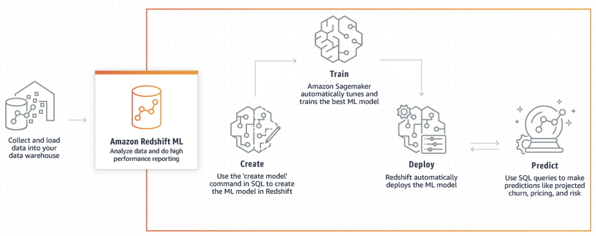
Solving a BinaryClassification ML problem: To determine how easy it is to make machine learning predictions with SQL on Redshift, I decided to create a machine learning model that is able to predict the possibility of retaining customers (churn) using the customer activity data.
This exercise makes use of the Orange Telecom Customer Churn Dataset available on Kaggle.
1. Data Preparation
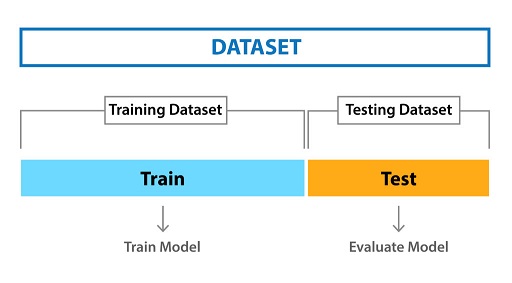
Splitting the dataset: after downloading the dataset from Kaggle, the first step is to prepare the data for use in a Redshift database. The data from Kaggle comes in two sets from the same batch but split in an 80/20 ratio as more data is often desirable for developing ML models.
- Train Set: used to train the model and is made up of 80% of the entire dataset.
- Test Set: to evaluate model performance, made up of 20% of the entire dataset.
We can implement the categorization of the data by combining the two datasets into one combined CSV spreadsheet and add an additional column called purpose with input values of train or test respectively as labels for both datasets. Out of the 3333 records available in our combined dataset, 2666 of the records will be used to train the model and the rest will be used for evaluation.
2. Setup Redshift Cluster
To get started with Amazon Redshift, we need to have a Redshift cluster setup for our data warehouse. Each cluster runs an Amazon Redshift engine and contains one or more databases.
From the AWS web console, navigate to the Amazon Redshift page from the list of services. Clicking on the Create cluster button will bring you to the page shown below. Input the cluster name (in this case, my cluster name is redshift-cluster-1) and workload type.
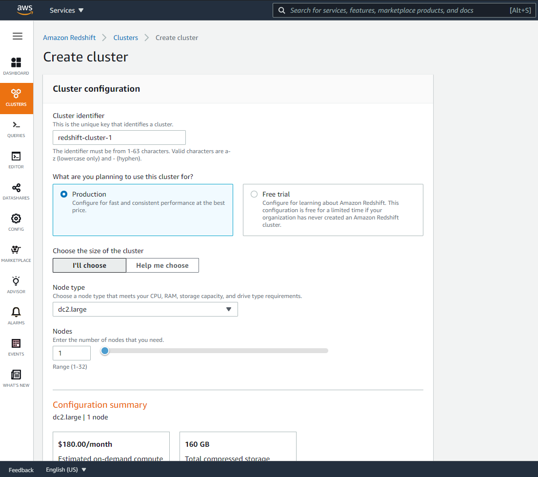
Redshift offers different node types to accommodate your workloads. For this exercise, I am selecting the smallest and cheapest node type dc2.large with a single node to save cost. You also need to set up a master username and password that will be used to authorize connectivity with the cluster after creation.
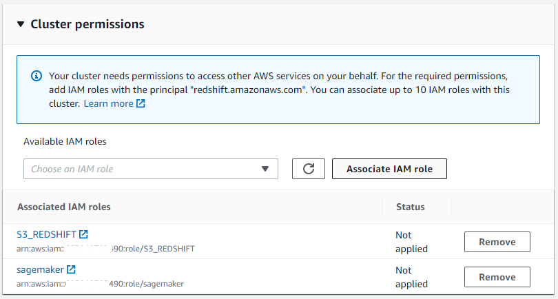
Working with Redshift ML requires necessary permissions to access other AWS services such as S3 and Sagemaker. You can associate up to 10 IAM roles to a single Redshift cluster.
3. Import Data To Redshift
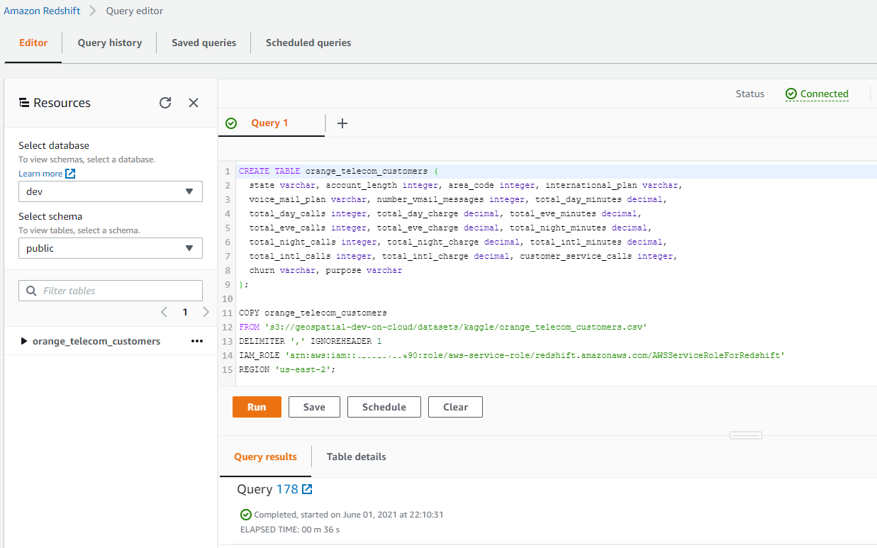
There are multiple ways of importing data into a Redshift database. For this exercise, we use the S3 method to import data to Redshift. First, we have to upload the prepared CSV data into an S3 bucket and then use the COPY command to import the data from S3 into a dedicated Redshift table.
The SQL code snippet below is responsible for creating a Redshift table to import our data into.
CREATE TABLE orange_telecom_customers (
  state varchar, account_length integer, area_code integer,
  international_plan varchar, voice_mail_plan varchar,
  number_vmail_messages integer, total_day_minutes decimal,
  total_day_calls integer, total_day_charge decimal,
  total_eve_minutes decimal, total_eve_calls integer,
  total_eve_charge decimal, total_night_minutes decimal,
  total_night_calls integer, total_night_charge decimal,
  total_intl_minutes decimal, total_intl_calls integer,
  total_intl_charge decimal, customer_service_calls integer,
  churn varchar, purpose varchar
);
After creating the Redshift table, we will then import the CSV data into it using the Redshifts COPY command.
COPY orange_telecom_customers
FROM 's3://geospatial-dev/redshift/orange_telecom_customers.csv'
DELIMITER ',' IGNOREHEADER 1
IAM_ROLE 'arn:aws:iam::XXXXXXXXXXXXX:role/RedshiftML'
REGION 'us-east-2';
4. Creating an ML Model
Amazon Redshift ML enables you to train models with a single SQL CREATE MODEL command. Once the data is imported, we can create and train our ML model based on this data.
To create a model in Redshift, use the Redshift ML CREATE MODEL statement.
CREATE MODEL orange_telecom_customers_model
FROM (SELECT
      state, account_length, area_code, international_plan, voice_mail_plan,
      number_vmail_messages, total_day_minutes, total_day_calls,
      total_day_charge, total_eve_minutes, total_eve_calls, total_eve_charge,
      total_night_minutes, total_night_calls, total_night_charge,
      total_intl_minutes, total_intl_calls, total_intl_charge,
      customer_service_calls, churn
      FROM orange_telecom_customers
      WHERE purpose = 'train'
  )
TARGET churn
FUNCTION ml_fn_orange_telecom_customers
IAM_ROLE 'arn:aws:iam::XXXXXXXXXXXXX:role/sagemaker'
SETTINGS (
  S3_BUCKET 'geospatial-dev'
);
In the above statement, we used SQL to select only the subset of our dataset that we've labeled for training purposes. For the TARGET variable we provided the name of the column we want to predict, which in this case is the churn column.
We also provided the name of the SQL function that will be generated after execution. Amazon Redshift will register the function as a SQL function for making predictions within your Amazon Redshift cluster. Other temporary data and training artifacts will be exported to the S3 Bucket provided in SETTINGS.
Depending on the size of the training dataset, it could take 45mins or more to finish training the model. Once the training is successful, you can visualize information about the model using the SQL command below.
SHOW MODEL orange_telecom_customers_model;
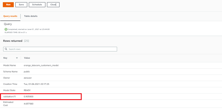
As highlighted in the image above, the F1 Score (used to analyze the accuracy for binary classification problems) for the model was 0.9038 which is quite an impressive outcome for a model that was created without machine knowledge or expertise.
The best part of doing machine learning with Redshift ML is the AutoML functionality. With AutoML in use, you don't have to know anything about the problem you are trying to solve or the best machine learning algorithm that applies. Redshift ML will automatically detect the problem type from the data and apply the best algorithm for training the model.
5. Making Predictions
Once the model is in a ready state, we can then use it for predictions by calling the function ml_fn_orange_telecom_customers that was generated during the model training process within our SQL commands.
For example, this SQL function can be used at the backend of the telecoms company applications to predict customers that are likely to churn in the future and use this knowledge to provide enticing offers/promos that could convince them to remain with the company.
SELECT churn,
       ml_fn_orange_telecom_customers(
          state, account_length, area_code, international_plan, voice_mail_plan,
          number_vmail_messages, total_day_minutes, total_day_calls,
          total_day_charge, total_eve_minutes, total_eve_calls, total_eve_charge,
          total_night_minutes, total_night_calls, total_night_charge,
          total_intl_minutes, total_intl_calls, total_intl_charge,
          customer_service_calls
       ) AS "prediction"
FROM orange_telecom_customers
WHERE purpose = 'test';
In the SQL command above, we used the function to make predictions on our test datasets. The output provides a side-by-side comparison of expected output churn and predicted output prediction.
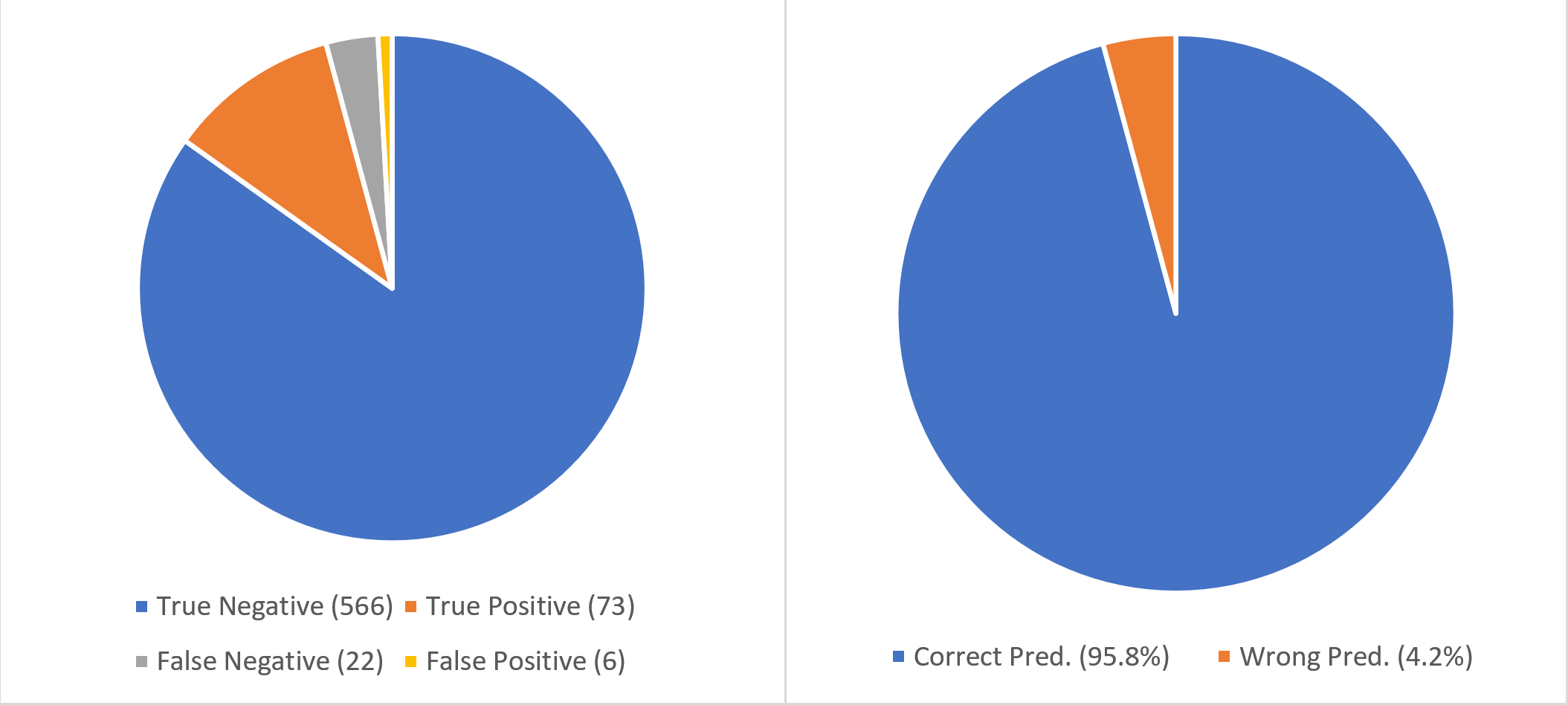
Prediction Report: On the test dataset, the model was able to achieve a 95% accuracy by making accurate predictions on 639 records out of 667 used in evaluating the model.
Problem type: BinaryClassification
Classification report:
              precision    recall  f1-score   support

       False       0.96      0.99      0.98       572
        True       0.92      0.77      0.84        95

    accuracy                           0.96       667
   macro avg       0.94      0.88      0.91       667
weighted avg       0.96      0.96      0.96       667

Accuracy Score: 0.9580209895052474
Area under curve: 0.8789657710710341
The report above shows that doing machine learning with Redshift produces the level of result or even better compared to creating custom Python models with frameworks like TensorFlow and PyTorch.
Conclusion
In conclusion, we saw how much of a game-changer Amazon Redshift ML is for organizations that can't afford the financial investment required to set up an in-house team of machine learning experts and resources but would like to apply machine learning knowledge to their datasets.
To learn more about using machine learning in Amazon Redshift, visit the AWS documentation page. You can also check out more of my articles at blog.somideolaoye.com.
